Comma.ai Calibration Challenge

Problem and objective

A forward-facing vehicle camera can be misaligned with the vehicle coordinate frame. The team investigated whether monocular video could be used to estimate the direction of motion—represented by pitch and yaw—and provide a signal for camera calibration.

The project combined geometric cues with learned temporal features: dense optical flow described motion between frames, vanishing-point geometry provided an interpretable reference, and a Conv-LSTM model mapped short image sequences to pitch and yaw estimates.

Motion and geometry cues

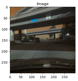
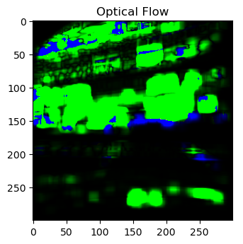
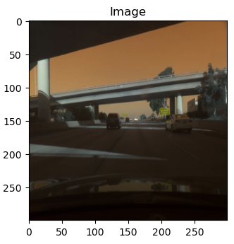
Dense optical flow

Farneback optical flow was computed between consecutive frames to approximate per-pixel motion. The horizontal and vertical flow fields were concatenated with RGB channels, producing a five-channel representation for one model configuration.

Vanishing-point estimate

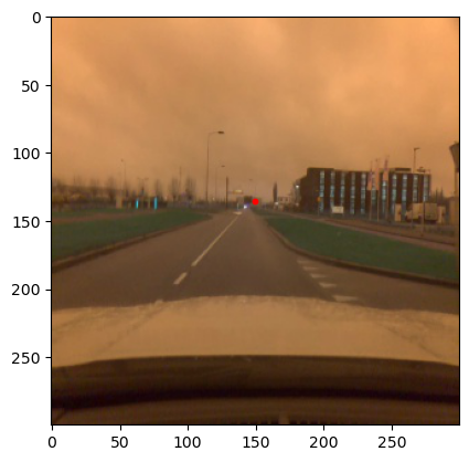
Parallel structures in the scene converge toward a vanishing point in the image plane. The team used this geometric cue to reason about the vehicle's direction of travel and its relationship to camera pitch and yaw.

Data pipeline

The dataset comprised five one-minute driving videos recorded at 20 frames per second. The team reported substantial missing labels and relatively few frames with meaningful directional change, so preprocessing was central to the experiment.

• Frame preparation: video was split into frames and resized to 256 × 256 pixels.
• Label continuity: missing pitch and yaw labels were interpolated for training sequences.
• Feature construction: RGB and optical-flow channels were evaluated separately and together.
• Temporal windows: sequences of 15 frames were used to expose short-term motion context.

Conv-LSTM architecture

Convolutional layers extracted spatial features from each frame, while LSTM layers modeled changes across the sequence. A final fully connected layer produced pitch and yaw predictions. The combined-input variant accepted RGB plus the two optical-flow components.

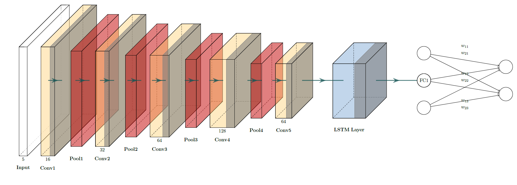
The reported training setup used 30 epochs, batches of 10 sequences, stochastic gradient descent, dropout, weight decay, and a weighted mean-squared-error objective intended to counter the imbalance between straight-driving and turning frames.

Experiment comparison

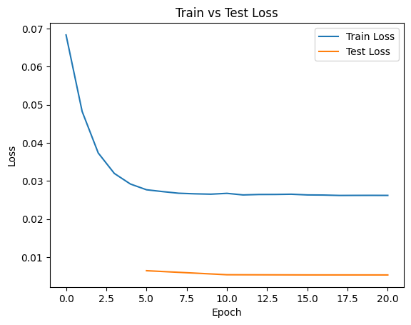
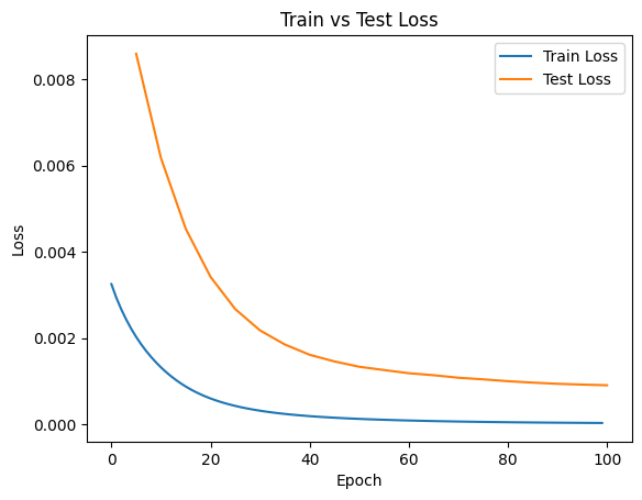
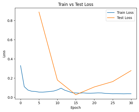
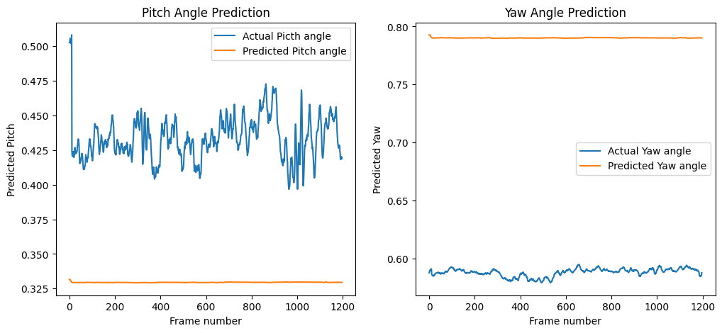
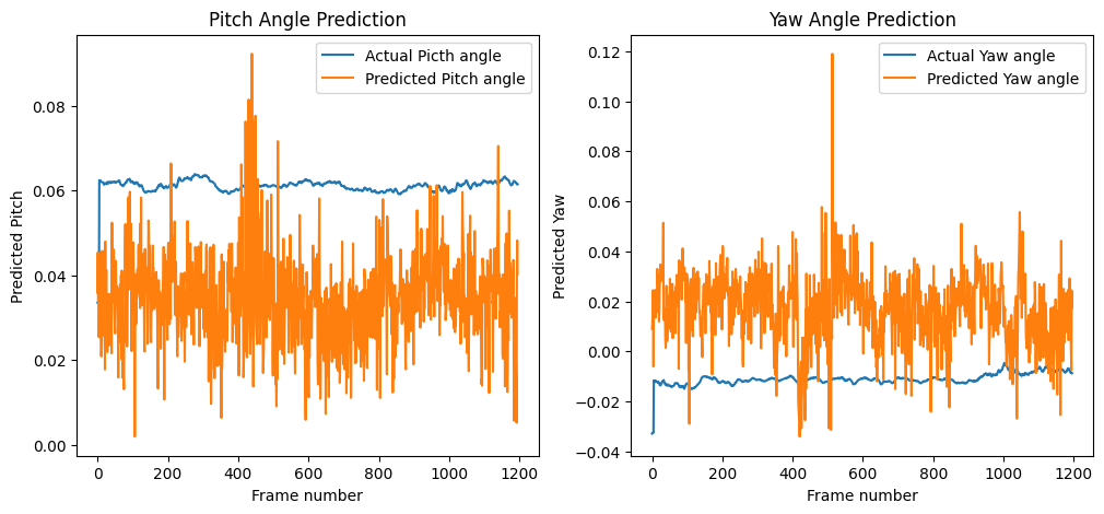
Three input configurations were compared: RGB frames alone, optical flow alone, and a fused RGB-plus-flow input. The loss curves below compare the three training configurations; they are not production benchmarks.

RGB only

Optical flow only

RGB and optical flow

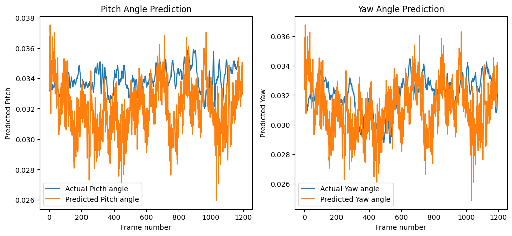
The fused representation captured both appearance and motion, but its predictions also showed higher variance. A plausible contributor was noise introduced by interpolated labels. Because the original summary did not define a reproducible denominator for its percentage-error claim, this page does not present that number as a validated metric.

Limitations and next steps

• Small, sparse dataset: a limited number of short videos restricted coverage of lighting, road geometry, and vehicle maneuvers.
• Interpolated supervision: filled labels improved continuity but may have introduced noise into the training target.
• Imbalanced motion: straight-driving frames dominated, making directional changes harder to learn.
• Offline features: precomputed dense flow added cost and did not establish real-time performance.

A stronger follow-up would define a held-out evaluation protocol, report angle errors in degrees with confidence intervals, test across distinct drives, and compare learned flow features with classical dense flow under the same runtime budget.